PANDAPandaor GIBBONGibbon?

A Beginner's Introduction to Adversarial Attacks
July 30, 2024

ABSTRACT

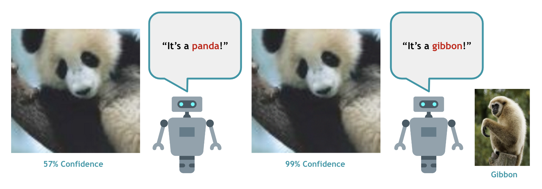
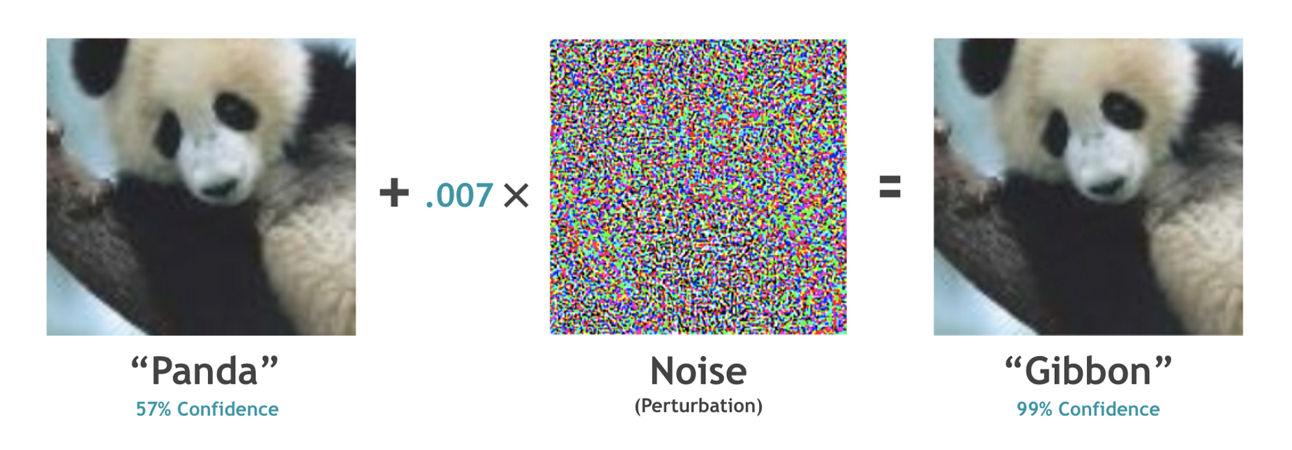
Though deep learning models have achieved remarkable success in diverse domains (e.g., facial recognition, autonomous driving), these models have been proven to be quite brittle to perturbations around the input data. Adversarial machine learning (AML) studies attacks that can fool machine learning models into generating incorrect outcomes as well as the defenses against worst-case attacks to strengthen model robustness. Specifically, for image classification, it is challenging to understand adversarial attacks due to their use of subtle perturbations that are not human-interpretable, as well as the variability of attack impacts influenced by attack methods, instance differences, or model architectures. This guide will utilize interactive visualizations to provide a non-expert introduction to adversarial attacks, and visualize the impact of FGSM attacks on two different ResNet-34 models. We designed this guide for beginners who are familiar with basic machine learning but new to advanced AML topics like adversarial attacks.

FROM THE BEGINNING

Before we use visualizations to understand the impacts of adversarial attacks on CNNs (yes, those are the soon-to-be data points you see floating on the right), let’s first go through the basics of adversarial attacks.

What is an Adversarial Attack?

In 2014, Goodfellow et al. [1] showed that an adversarial image of a panda could fool GoogLeNet into classifying it as a gibbon with high confidence, leading to the birth of AML research. An adversarial "evasion" attack produces adversarial examples that are crafted with small, indistinguishable perturbations with the goal of causing model prediction errors, such as image misclassifications.

What is an FGSM Attack?

The panda attack you just saw is called the Fast Gradient Sign Method (FGSM) attack, one of the first and most well-known adversarial attacks. It is a white-box attack (i.e., the attacker has access to model internals) that adjusts the input image by taking a step in the direction of the sign of the backpropagated gradients.

The idea is to manipulate the input data to maximize the loss, instead of minimizing it like we do during model training. In other words, it makes small changes to the input image to push the model to make a wrong prediction:
x=x+ϵsign(xJ(θ,x,y)).\mathbf{x}' = \mathbf{x} +\epsilon \textrm{\textrm{sign}}(\nabla_{\mathbf{x}} J(\theta, \mathbf{x}, y)).

Specifically,

  • x\mathbf{x}' : This is the adversarial image.
  • x\mathbf{x} : This is the original input image.
  • J(θ,x,y)J(\theta, \mathbf{x}, y) : This is the loss function that measures how far the model’s predictions are from the true label yy . It depends on the model’s parameters θ\theta , the input image x\mathbf{x} , and the true label yy .
  • xJ(θ,x,y)\nabla_{\mathbf{x}} J(\theta, \mathbf{x}, y) : This is the gradient of the loss function w.r.t the input image. It tells the attacker in which direction the input should be changed to increase the loss.
  • sign(xJ(θ,x,y))\textrm{sign}(\nabla_{\mathbf{x}} J(\theta, \mathbf{x}, y)) : This extracts the direction (+ or -) of the gradient, indicating whether each pixel should be increased or decreased to result in model error.
  • ϵ\epsilon : This controls the magnitude of the perturbation. If ϵ\epsilon is too large, the changes become too noticeable to humans; if too small, the attack might not be effective.

In short, the FGSM attack creates an adversarial image by adding a small amount of perturbation to the original image in the direction that increases the model’s loss. This perturbation ϵ\epsilon is enough to fool machine learning models, but usually so subtle that a human wouldn’t really notice them.

How does the CNN see a gibbon then?

While the attack logic is simple and intuitive, how can two panda images that appear indistinguishable to humans seem so different to machine learning models?

Let's examine how the FGSM attack alters a CNN's perception of image datasets.

DATASET & MODEL

CIFAR-10 Dataset

On the right, we have loaded 100 sampled images from the CIFAR-10 dataset [2] in the scatterplot. The CIFAR-10 dataset consists of 60,000 (32 × 32) colored images from 10 different classes (50,000 training data and 10,000 testing data), with 6,000 images per class. Here, we randomly sampled 10 images from each class.

We use the following colors to represent these classes:

Each circle in the scatterplot represents an instance from the dataset and is split into two halves: the color of the left half represents its ground truth label, while the color of the right half represents the model's prediction of the image.

ResNet-34 Model

For this article, we will use the ResNet-34 model and start by visualizing its perception of the CIFAR-10 dataset by extracting its embeddings.

ResNet-34[3] is a convolutional neural network (CNN) that is part of the Residual Networks family, which utilizes residual learning. In traditional DNNs, each layer learns a full transformation from the input to the desired output. However, as networks become deeper, training becomes more challenging due to problems like the vanishing gradient problem.

Residual learning addresses this by focusing on the residual — the difference between the desired layer output and what earlier layers produced. This way, each layer only learns what to add to the previous output. This is done through skip connections that pass one layer’s output directly to later layers. The architecture we selected consists of 34 layers and is widely adopted for its strong performance in image classification.


To extract ResNet-34′s perception of the images, we temporarily detach the final output layer to obtain the embeddings, which are high-dimensional representations capturing the essential features of the input images.

Exploring the Data Points

Start exploring the data points by hovering over them and observing their ground truth labels and ResNet-34's predictions.

INTERACTING WITH DATA POINTS

Projecting onto a 2-D Space

To reveal important patterns in the embeddings and transform them into a format that can be easily visualized, we apply dimensionality reduction to project the model embeddings into a lower dimension. We start by using t-SNE (t-distributed Stochastic Neighbor Embedding) [4].

t-SNE works by converting similarities between data points into probabilities and then maps these points into a 2-D space while preserving the relative distances. It highlights clusters and relationships in the data that aren’t easily seen in higher dimensions.

The resulting outputs are scaled to be used as the x- and y-coordinates of the instances in the scatterplot shown on the right.

Note: although t-SNE is a powerful tool and often produces visually impressive results [7][8], it does come with certain limitations and must be used cautiously.

  • Sensitivity to initialization [9]: t-SNE’s produced results can vary based on its initial conditions, which means that different runs could potentially produce different results. In our case, we average the results from multiple runs to create a more stable and reliable representation.
  • Local linearity assumption [10]: t-SNE relies on the assumption of local linearity, which may not always hold true. This may lead to distortions in how global data structures are represented in the 2-D space.
  • Limited clustering capabilities [11]: t-SNE may only partially recover clusters under special circumstances. Visualized clusters should be interpreted cautiously, as they may not directly correspond to clusters in the original high-dimensional space.
  • Class-cluster assumption [12]: One should not assume that classes in high-dimensional data will always manifest as distinct clusters in t-SNE’s representation. The aglorithm highights local structures but may be misleading when interpreting global patterns.

Given these caveats, it is important to use t-SNE cautiously in less well-studied use cases.

Visualizing the Rest of the Dataset

To further visualize the global distribution of ResNet-34′s embeddings on the entire CIFAR-10 dataset (with 10,000 images), we also include a hexagonal binning backdrop in our scatterplot. This helps provide context even when only a subset of the dataset is actively displayed.

The hexbin map shows the global distribution of the entire dataset, regardless of how many data points are visible in the foreground. Each hexagon is colored according to the model’s predicted class, and the size of the hexagon represents the frequency of instances being predicted as that class in that region. We use hexbins instead of circles here because using circles for all data points would lead to significant visual clutter, making the scatterplot harder to interpret.

By employing hexagons, we can aggregate the data into manageable regions, reducing visual noise and providing a clearer view of the overall distribution. This way, the map shows the general trends in clustering based on model predictions, allowing for quick identification of decision boundaries and similarly classified image groups.

Exploring the Embedding Distribution

With the help of the hexbin backdrop, take a look at the spatial distribution of ResNet-34′s embeddings projected by t-SNE. What can you learn about ResNet-34′s perception of the natural CIFAR-10 dataset?

From the projection, we can see that the CIFAR-10 embeddings of ResNet-34 form small, distinct class clusters. When no attack has been conducted, most of the confusion seems to happen within the center of the projection, near the “boundaries” of the distinct clusters. Overall, ResNet-34 achieves high accuracy.

However, something that may catch your attention is that, although a closer distance between instances generally means that the model perceives them as “more similar,” we can see that there are classes that we don’t deem similar at all close to each other, e.g., birds and automobiles.

CONDUCTING THE ATTACK

Applying Perturbations

Previously, we introduced the FGSM attack [1], which generates perturbations to craft adversarial examples. Perturbation refers to small, often imperceptible changes made to input data with the intent to mislead models into making incorrect predictions.

Here, we utilize the FGSM attack with the LL^{\infty} norm to generate adversarial examples.

FGSM with L-infinity

Also known as the Chebyshev distance, the LL^{\infty} distance is commonly adapted by adversarial attacks to generate perturbed images by measuring the maximum pixel difference between two images. For example, if x\mathbf{x} is the original image input, and x=x+n\mathbf{x}' = \mathbf{x} + \mathbf{n} is the adversarial output where n\mathbf{n} is equivalent to ϵsign(xJ(θ,x,y))\epsilon \cdot \text{sign}(\nabla_{\mathbf{x}} J(\theta, \mathbf{x}, y)) , then the LL^{\infty} distance between x\mathbf{x} and x\mathbf{x}' is computed as the following:

n=maxini.||\mathbf{n}||_{\infty} = \max_{i} |n_i|.
  • n\mathbf{n} : This represents the perturbation added to the original image. Every element in n\mathbf{n} corresponds to the value change in a specific pixel.
  • ni|n_i| : The absolute value of the change for pixel ii , where ii indicates the pixel index.
  • maxini\max_i |n_i| : This is the maximum absolute value of the perturbations applied to the image. It means looking at all the pixel changes and identify the one that is the largest.
  • n||\mathbf{n}||_{\infty} : This is the notation for the LL^{\infty} norm.

(Use the slider below to adjust ϵ\epsilon and observe the changes in ResNet-34′s embeddings.)


Now, we will apply these perturbations to our data points to observe their effects.

None 0.03
Perturbation Size (ε): 0.00

Accuracy vs. Robustness

In AML, accuracy (or natural accuracy) refers to the model’s performance on clean data, while robustness (or robust accuracy) measures its performance on adversarially perturbed data. Check the bar chart below to see how accuracy on the entire dataset drops after applying perturbations.

Exploring Dataset-level Attack Impact

Adjust the slider and observe the changes in model embeddings and prediction accuracy. What interesting insights can you find?

When the perturbation size is set to values above 0, the data points within the scatterplot start to move rapidly, mostly towards the center of the plot. This suggests that the FGSM attack has drastically altered ResNet-34′s perception of these images’ features.

As the perturbation size increases, ResNet-34′s prediction accuracy continues to drop, eventually reaching 57% at a perturbation size of 0.03.

Is It Imperceptible?

To investigate specific images before and after the attack, adjust the perturbation slider above, then click on a data point in the embeddings and observe the natural and adversarial images below.

Ground Truth Label
Original Prediction
Current Prediction
Panda
Panda
Gibbon
Loading...

Can you spot the differences between the natural and adversarial images?

The larger the perturbation size, the more obvious the perturbations are and the more effective the attack is. That’s why attackers aim to find a middle point where the perturbations are subtle yet sufficient to lead to a misclassification. However, keep in mind that the CIFAR-10 dataset consists of 32 × 32 images, so the applied noise is relatively more apparent compared to high-resolution images (e.g., the panda image).

ADVERSARIAL TRAINING

Training ResNet-34 Differently

Now, let’s take a look at a different ResNet-34. (Let’s call it ResNet-34★.)

On the right, we have loaded the CIFAR-10 embeddings of this new ResNet-34 when no attack has been conducted. This ResNet-34★ shares the same model architecture as the previous ResNet-34 we just explored, but it has been specifically trained with adversarial training (AT) [5].

What is Adversarial Training (AT)?

To counter adversarial attacks, various defense methods have been proposed to fortify model robustness against adversarial inputs. Adversarial training is currently the most effective defense, which trains classifiers with adversarial examples by adding them to the training set or through regularizations.

Here, we use TRadeoff-inspired Adversarial DEfense via Surrogate-loss minimization (TRADES)[6] to train ResNet-34★, one of the state-of-the-art adversarial training methods.

What is TRADES?

TRADES[6] is an advanced AT method designed to enhance the robustness of neural networks against adversarial attacks. It focuses on balancing the trade-off between accuracy on unperturbed data and robustness against adversarial examples by introducing a surrogate loss function. This surrogate loss penalizes large deviations in predictions caused by small perturbations, ensuring that a model that can maintain relatively high natural accuracy while being resilient to adversarial manipulations.

Specifically, TRADES uses the following optimization problem for the loss function: minfE{L(f(X),Y)+βmaxXBall(X,ϵ)L(f(X),f(X))}\min_{f} \mathbb{E} \left\{ \mathcal{L}(f(X), Y) + \beta \max_{X' \in \mathsf{Ball}(X, \epsilon)} \mathcal{L}(f(X), f(X')) \right\}

  • minf\min_f means we are finding the function ff that minimizes the overall loss.
  • E{...}\mathbb{E}\{...\} represents the expected value, meaning that we are minimizing the average loss over all inputs from the dataset.
  • L(f(X),Y)L(f(X),Y) is the first part of the loss function; it represents the standard classification loss, which measures how well the model’s predictions on the clean data (i.e., f(X)f(X) ) match true labels YY .
  • β\beta balances between the standard classification loss and the adversarial loss. A larger β\beta emphasizes on robustness, while a smaller β\beta prioritizes natural accuracy.
  • maxXBall(X,ϵ)L(f(X),f(X))\max_{X' \in \text{Ball}(X, \epsilon)} L(f(X),f(X')) is the second part of the loss; it looks for an adversarial example XX' within a perturbation ϵ\epsilon of XX . It measures how different the model’s predictions are for the clean and adversarial examples. The goal is to ensure that the predictions for XX and XX' are as close as possible.

To summarize:

  1. The first part of TRADE’s loss ensures the model performs well on clean data (i.e., natural accuracy).
  2. The second part prevents the model from changing its prediction too much when the input is perturbed by an attack (i.e., adversarial robustness).

Applying Perturbations Again

Now, let’s try conducting the FGSM attack on ResNet-34★ and see what happens.

None 0.03
Perturbation Size (ε): 0.00

What do you notice about ResNet-34★'s behavior compared to ResNet-34's?

Compared to the naturally trained ResNet-34, the FGSM attack barely changes how ResNet-34★ perceives the CIFAR-10 dataset (as the data points are barely moving). Hence, ResNet-34★ achieves higher robustness than ResNet-34.

How Come the Difference?

Why does the FGSM attack drastically alter the features extracted by ResNet-34 from the CIFAR-10 dataset, but not those extracted by ResNet-34★?

To understand this, let’s closely examine the noises generated by FGSM for both ResNet-34 and ResNet-34★. Keep in mind that these noises are based on the gradient of the loss function, shedding light on the features each model relies on most for their predictions.

Click on a data point and observe the perturbations generated by FGSM for ResNet-34 versus ResNet-34★.


What do you notice about the noises?

Compared to the noises generated for ResNet-34, the noises generated for ResNet-34★ have more defined shapes that resemble the original images. Since these noises are gradient-based, this suggests that ResNet-34★ relies on more human-interpretable features for classification, making it more robust.

SUMMARY & CONCLUSION

In this guide, we explored adversarial attacks on CNNs, focusing on the FGSM attack and its impact on ResNet-34 models. We demonstrated how subtle perturbations can lead to significant misclassifications.

What We Learned

1. Adversarial Attacks: Small, intentional changes to input data can deceive models into incorrect predictions. FGSM is a simple yet effective method to generate such adversarial examples.

2. Impact on Models: Applying FGSM showed a drastic drop in model accuracy with increasing perturbation size, highlighting the vulnerability of models to adversarial attacks.

3. Adversarial Training (AT): TRADES, an advanced adversarial training method, balances accuracy and robustness, enhancing model resilience against adversarial perturbations.

4. Model Comparisons: ResNet-34★, trained with TRADES, demonstrated higher robustness to FGSM attacks compared to the naturally trained ResNet-34.

Understanding adversarial attacks and defenses is important for developing robust AI systems. By integrating advanced training techniques, we can build models that are both accurate and robust to adversarial manipulations, ensuring their reliability in real-world applications.

Learn More About Adversarial Attacks

If you are interested in exploring adversarial attacks and related topics further, here are some other online resources:

  1. TensorFlow Tutorial - Adversarial Attacks Using FGSM (link)
  2. Pytorch Tutorial - Adversarial Example Generation (link)
  3. SEI Blog (Carnegie Mellon University) - The Challenge of Adversarial Machine Learning (link)
  4. AdVis.js - Exploring Fast Gradient Sign Method (link)
  5. Bluff - Interactively Deciphering Adversarial Attacks on Deep Neural Networks (link)

References

  1. Explaining and harnessing adversarial examples.
    Goodfellow, Ian J and Shlens, Jonathon and Szegedy, Christian.
    arXiv preprint arXiv:1412.6572, 2014.
  2. Learning Multiple Layers of Features from Tiny Images.
    Krizhevsky, A.
    Master's thesis, University of Toronto, 2009.
  3. Deep residual learning for image recognition.
    He, Kaiming and Zhang, Xiangyu and Ren, Shaoqing and Sun, Jian.
    Proceedings of the IEEE conference on computer vision and pattern recognition, 2016.
  4. Visualizing data using t-SNE.
    Van der Maaten, Laurens and Hinton, Geoffrey.
    Journal of machine learning research, 2008.
  5. Towards deep learning models resistant to adversarial attacks.
    Madry, Aleksander and Makelov, Aleksandar and Schmidt, Ludwig and Tsipras, Dimitris and Vladu, Adrian.
    arXiv preprint arXiv:1706.06083, 2017.
  6. Theoretically principled trade-off between robustness and accuracy.
    Zhang, Hongyang and Yu, Yaodong and Jiao, Jiantao and Xing, Eric and El Ghaoui, Laurent and Jordan, Michael.
    International conference on machine learning, 2019.
  7. Toward a quantitative survey of dimension reduction techniques.
    Espadoto, Mateus and Martins, Rafael M and Kerren, Andreas and Hirata, Nina ST and Telea, Alexandru C.
    IEEE transactions on visualization and computer graphics, 2019.
  8. Large-scale evaluation of topic models and dimensionality reduction methods for 2d text spatialization.
    Atzberger, Daniel and Cech, Tim and Trapp, Matthias and Richter, Rico and Scheibel, Willy and D{"o}llner, Jurgen and Schreck, Tobias.
    IEEE Transactions on Visualization and Computer Graphics, 2023.
  9. Initialization is critical for preserving global data structure in both t-SNE and UMAP.
    Kobak, Dmitry and Linderman, George C.
    Nature biotechnology, 2021.
  10. Visualizing data using t-sne.
    vd Maaten, Laurens and Hinton, Geoffrey.
    Journal of machine learning research, 2008.
  11. An analysis of the t-sne algorithm for data visualization.
    Arora, Sanjeev and Hu, Wei and Kothari, Pravesh K.
    Conference on learning theory, 2018.
  12. Classes are not clusters: Improving label-based evaluation of dimensionality reduction.
    Jeon, Hyeon and Kuo, Yun-Hsin and Ma, Kwan-Liu and Seo, Jinwook and others.
    IEEE Transactions on Visualization and Computer Graphics, 2023.